5.1. The standard cosmological model

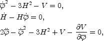
The standard model of cosmological evolution rests on three important assumptions [100]. The first assumption is that over very large length scales (greater than 50 Mpc) the Universe is described by a homogeneous and isotropic Friedmann-Robertson-Walker (FRW) line element:

(5.1)

where a() is the scale factor and the conformal-time coordinate (notice that Eq. (5.1) has been written, for simplicity, in the conformally flat case). The second hypothesis is that the sources of the evolution of the background geometry are perfect fluid sources. As a consequence the entropy of the sources is constant. The third and final hypothesis is that the dynamics of the sources and of the geometry is dictated by the general relativistic FRW equations ⁽¹⁶⁾:

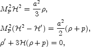(5.2) (5.3) (5.4)

where = (ln a)' and the prime ⁽¹⁷⁾ denotes the derivation with respect to . Recall also, for notational convenience, that aH = where H = / a is the conventional Hubble parameter. The various tests of the standard cosmological model are well known [101, 102]. Probably one of the most stringent one comes from the possible distortions, in the Rayleigh-Jeans region, of the CMB spectrum. The absence of these distortions clearly rules out steady-state cosmological models. In the standard cosmological model one usually defines the proper distance of the event horizon at the time t₁

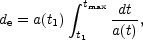(5.5)

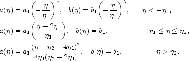
this distance represents the maximal extension of the region over which causal connection is possible. Furthermore, the proper distance of the particle horizon can also be defined:

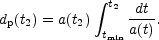(5.6)

If the scale factor is parametrized as a(t) ~ t, for 0 < < 1 the Universe experiences a decelerated expansion, i.e. > 0 and < 0 while the curvature scale decreases, i.e. < 0. This is the peculiar behaviour when the fluid sources are dominated either by dust (p = 0) or by radiation (p = / 3). In the case of the standard model, the particle horizon increases linearly in cosmic time (therefore faster than the scale factor). This implies that the CMB radiation, today observed with a temperature of 2.7K over the whole present horizon has been emitted from space-time regions which were not in causal contact. This problem is known as the horizon problem of the standard cosmological model. The other problem of the standard model is related to the fact that today the intrinsic (spatial) curvature k / a² is smaller than the extrinsic curvature, i.e. H². Recalling that k / (a² H²) = k / ² it is clear that if < 0, 1 / ² increases so that the intrinsic curvature could be, today, arbitrarily large. The third problem of the standard cosmological model is related to the generation of the large entropy of the present Universe. The solution of the kinematical problems of the standard model is usually discussed in the framework of a phase of accelerated expansion [103], i.e. > 0 and > 0. In the case of inflationary dynamics the extension of the causally connected regions grows as the scale factor and hence faster than in the decelerated phase. This solves the horizon problem. Furthermore, during inflation the contribution of the spatial curvature becomes very small. The way inflation solves the curvature problem is by producing a very tiny spatial curvature at the onset of the radiation epoch taking place right after inflation. The spatial curvature can well grow during the decelerated phase of expansion but is will be always subleading provided inflation lasted for sufficiently long time. In fact, the minimal requirement in order to solve these problems is that inflation lasts, at least, 60-efolds. The final quantity which has to be introduced is the Hubble radius H^-1(t). This quantity is local in time, however, a sloppy nomenclature often exchanges the Hubble radius with the horizon. Since this terminology is rather common, it will also be used here. In the following applications it will be relevant to recall some of the useful thermodynamical relations. 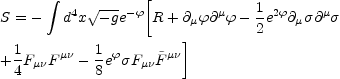In particular, in radiation dominated Universe, the relation between the Hubble parameter and the temperature is given by

(5.7)

where g_* is the effective number of relativistic degrees of freedom at the corresponding temperature. Eq. (5.2), implying H² M_P² = / 3, has been used in Eq. (5.7) together with the known relations valid in a radiation dominated background

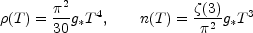(5.8)

where (3) 1.2. In Eq. 5.8) the thermodynamical relation for the number density n(T) has been also introduced for future convenience.

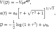
5.1.1. Inflationary dynamics and its extensions

The inflationary dynamics can be realized in different ways. Conventional inflationary models are based either on one single inflaton field [104, 105, 106, 107] or on various fields [108] (see [109] for a review). Furthermore, in the context of single-field inflationary models one oughts to distinguish between small-field models [106] (like in the so-called new-inflationary models) and large-field models [107] (like in the case of chaotic models).

In spite of their various quantitative differences, conventional inflationary models are based on the idea that during the phase of accelerated expansion the curvature scale is approximately constant (or slightly decreasing). After inflation, the radiation dominated phase starts. It is sometimes useful for numerical estimates to assume that radiation suddenly dominates at the end of inflation. In this case the scale factor can be written as

(5.9)

where is some effective exponent parameterizing the dynamics of the primordial phase of the Universe. Notice that if = 1 we have that the primordial phase coincides with a de Sitter inflationary epoch. The case = 1 is not completely realistic since it corresponds to the case where the energy-momentum tensor is simply given by a (constant) cosmological term. In this case the scalar fluctuations of the geometry are not amplified and the large-scale angular anisotropy in the CMB would not be reproduced. The idea is then to discuss more realistic energy-momentum tensors leading to a dynamical behaviour close to the one of pure de Sitter space, hence the name quasi-de Sitter space-times. Quasi-de Sitter dynamics can be realized in different ways. One possibility is to demand that the inflaton slowly rolls down from its potential obeying the approximate equations

(5.10)

valid provided ₁ = - / H² << 1 and ₂ = / (H ) << 1. There also exist exact inflationary solutions like the power-law solutions obtainable in the case of exponential potentials:

(5.11)

Since, from the exact equations, 2M_P² = -² the two slow-roll parameters can also be written as

(5.12)

In the case of the exponential potential (5.11) the slow-roll parameters are all equal, ₁ = ₂ = 1 / p. Typical potentials leading to the usual inflationary dynamics are power-law potentials of the type V() ⁿ, exponential potentials, trigonometric potentials and nearly any potential satisfying, in some region of the parameter space, the slow-roll conditions.

Inflation can also be realized in the case when the curvature scale is increasing, i.e. > 0 and > 0. This is the case of superinflationary dynamics. For instance the propagation of fundamental strings in curved backgrounds [110, 111] may lead to superinflationary solutions [113, 114]. A particularly simple case of superinflationary solutions arises in the case when internal dimensions are present.

Consider a homogeneous and anisotropic manifold whose line element can be written as

(5.13)

[ is the conformal time coordinate related, as usual to the cosmic time t = a() d ; _ij(x), _ab(y) are the metric tensors of two maximally symmetric Euclidean manifolds parameterized, respectively, by the "internal" and the "external" coordinates {xⁱ} and {y^a}]. The metric of Eq. (5.13) describes the situation in which the d external dimensions (evolving with scale factor a()) and the n internal ones (evolving with scale factor b()) are dynamically decoupled from each other [115].

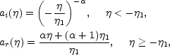
A model of background evolution can be generically written as

(5.14)

In the parameterization of Eq. (5.14) the internal dimensions grow (in conformal time) for < 0 and they shrink for > 0 ⁽¹⁸⁾.

Superinflationary solutions are also common in the context of the low-energy string effective action [119, 120, 121]. In critical superstring theory the electromagnetic field F_µ is coupled not only to the metric (g_µ), but also to the dilaton background (). In the low energy limit such interaction is represented by the string effective action [119, 120, 121], which reads, after reduction from ten to four expanding dimensions,

(5.15)

were = - ln V₆ ln(g²) controls the tree-level four-dimensional gauge coupling ( being the ten-dimensional dilaton field, and V₆ the volume of the six-dimensional compact internal space). The field is the Kalb-Ramond axion whose pseudoscalar coupling to the gauge fields may also be interesting.

In the inflationary models based on the above effective action [122, 123] the dilaton background is not at all constant, but undergoes an accelerated evolution from the string perturbative vacuum ( = - ) towards the strong coupling regime, where it is expected to remain frozen at its present value. The peculiar feature of this string cosmological scenario (sometimes called pre-big bang [123]) is that not only the curvature evolves but also the gauge coupling. Suppose, for the moment that the gauge fields are set to zero. The phase of growing curvature and dilaton coupling (< > 0, > 0), driven by the kinetic energy of the dilaton field, is correctly described in terms of the lowest order string effective action only up to the conformal time = _s at which the curvature reaches the string scale H_s = _s^-1 (_s (')^1/2 is the fundamental length of string theory). A first important parameter of this cosmological model is thus the value _s attained by the dilaton at = _s. Provided such value is sufficiently negative (i.e. provided the coupling g = e^/2 is sufficiently small to be still in the perturbative region at = _s), it is also arbitrary, since there is no perturbative potential to break invariance under shifts of . For > _s high-derivatives terms (higher orders in ') become important in the string effective action, and the background enters a genuinely "stringy" phase of unknown duration. An assumption of string cosmology is that the stringy phase eventually ends at some conformal time ₁ in the strong coupling regime. At this time the dilaton, feeling a non-trivial potential, freezes to its present constant value = ₁ and the standard radiation-dominated era starts. The total duration ₁ / _s, or the total red-shift z_s encountered during the stringy epoch (i.e. between _s and ₁), will be the second crucial parameter besides _s entering our discussion. For the purpose of this paper, two parameters are enough to specify completely our model of background, if we accept that during the string phase the curvature stays controlled by the string scale, that is H g M_{P s}^-1 (M_p is the Planck mass) for _s < < ₁.

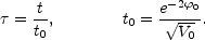
During the string era and H are approximately constant, while, during the dilaton-driven epoch

(5.16)

Here _{i i}² represents the possible effect of internal dimensions whose radii b_i shrink like (- t)^_i for t 0_- (for the sake of definiteness we show in the figure the case = 0). The shape of the coupling curve corresponds to the fact that the dilaton is constant during the radiation era, that is approximately constant during the string era, and that it evolves like

(5.17)

during the dilaton-driven era.

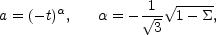
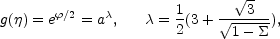
An interesting possibility, in the pre-big bang context is that the exit to the phase of decelerated expansion and decreasing curvature takes place without any string tension correction. Recently a model of this kind has been proposed [124]. The idea consists in adding a non-local dilaton potential which is invariant under scale factor duality. The evolution equations of the metric and of the dilaton will then become, in 4 space-time dimensions,

(5.18)

where = - 3 log a is the shifted dilaton. A particular solution to these equations will be given by

(5.19) (5.20) (5.21)

where

(5.22)

This solution interpolates smoothly between two self-dual solutions. For t - the background superinflates while for t + the decelerated FRW limit is recovered.

¹⁶ Units M_P = (8 G)^-1/2 = 1.72 × 10¹⁸ GeV will be used. Back.

¹⁷ The overdot will usually denote derivation with respect to the cosmic time coordinate t related to conformal time as dt = a() d. Back.

¹⁸ To assume that the internal dimensions are constant during the radiation and matter dominated epoch is not strictly necessary. If the internal dimensions have a time variation during the radiation phase we must anyway impose the BBN bounds on their variation [116, 117, 118]. The tiny variation allowed by BBN implies that b() must be effectively constant for practical purposes. Back.