15.9. COSMOLOGY MADE SIMPLE: THE SHELL MODEL

The evolutionary models described in Section 15.5 are based on complex numerical calculations that tend to obscure connections between important features in the data and the calculated radio luminosity functions, redshift distributions, etc. In contrast, von Hoerner (1973) demonstrated with analytic approximations the importance of the broad visibility function (Equation 15.14) to the radio Hubble relation and to the form of the source count. In a uniformly filled, static Euclidean universe, the visibility function has no effect on the form of the source count (Equation 15.16) or the Hubble relation. The visibility function is important only if its width, log L, is greater than twice the redshift range, log z, containing most radio sources. Thus, the actual distribution of extragalactic radio sources in distance (lookback time) is so nonuniform that features in the source counts should not be interpreted as perturbations from a static Euclidean count. A much better starting model for the radio universe is actually a hollow shell centered on the observer! This "shell model" reproduces many features of the data almost as well as the more elaborate models and clearly shows how they are related to the distribution of sources in space.

For sources with average spectral index <> the relation

(15.30)

is a good approximation to the exact Equations (15.20) and (15.21) for all 0 2, z < 5 (Condon 1984a). If most radio sources are confined to a thin shell of thickness z_s at redshift z_s,

(15.31)

We assume translation evolution so _m(L| z, ) = g(z) _m[L / f (z)| z = 0, ]. Let g_s g(z_s) be the amount of density evolution and f_s f (z_s) be the amount of luminosity evolution at the shell redshift. Then, log[(L | z_s, )] = log[(L / f_s| z = O, )] + 3 log(f_s) / 2 + log(g_s) and

(15.32)

The redshift distribution of sources stronger than S = 2 at = 1.4 GHz (Figure 15.9) suggests z_s 0.8 and ( z_s / z_s) 1 ; the spectral-index distribution [Figure 15.7(b)] gives <> 0.7. Substituting these quantities yields the following expression relating the weighted source counts, the local visibility function, and the evolution parameters at the shell redshift:

(15.33)

The values of f_s and g_s that satisfy Equation (15.33) can be found graphically by superimposing the observed source counts and local visibility functions, as shown in Figure 15.17. For sources with z_m 0.8 and 0.7, log[L(W Hz^-1)] - log[S(Jy)] 26.9. Since the best fit of the local visibility function to the source counts occurs at log[L(W Hz^-1)] - log[S(Jy)] 25.7 (Figure 15.17), we require luminosity evolution in the amount log(f_s) 26.9 - 25.7 = 1.2. This fit also implies log[S^5/2 n(S | = 1.4 GHz)] log[(L | z = 0, = 1.4 GHz)] - 0.65, resulting in log(g_s) 0.0 (no density evolution). With these evolution parameters, the weighted source count predicted by the shell model corresponds exactly to the local visibility function plotted as the solid line in Figure 15.17. The model actually reproduces the entire observed source count from S 10µJy to S 10 Ky.

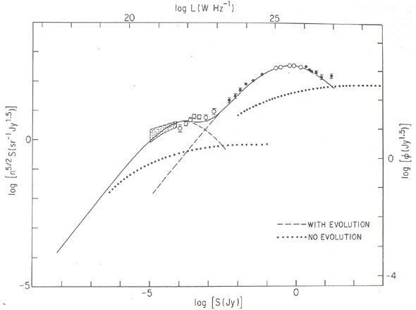Figure 15.17. Superposition of the weighted source count at 1.4 GHz (data points) and the hyperbolic fits to the 1.4-GHz local visibility functions for radio sources in spiral and elliptical galaxies (dashed lines). The combined local visibility function for all radio sources is indicated by the solid curve. This curve also plots the weighted source count predicted by the shell model. The source counts expected from nonevolving populations of spiral and elliptical galaxies described by this local luminosity function are shown as dotted curves. Lower abscissa: log flux density (Jy). Left ordinate: log weighted source counts (sr-1 (Jy1.5). Upper abscissa: log spectral luminosity (W Hz-1). Right ordinate: log weighted luminosity function Jy1.5).

Since the shell model ignores local sources, it must fail at the highest flux densities - the regime in which a nonevolving model is more appropriate. What is surprising is that the transition flux density is so high. An exact calculation based on the same local luminosity function without evolution yields log[S^5/2 n(S | = 1.4 GHz)] 1.8 at high flux densities (Figure 15.17), so the shell model and the nonevolving model predict the same source counts at S 20 Jy. Thus, the static Euclidean approximation is reasonably good only for S > 20 Jy at = 1.4 GHz; it applies only to the small number of sources in the very strongest flux-density bin plotted in Figure 15.17. It should not be used to describe features in the observed counts at lower flux densities. For example, the so-called "Euclidean" regions in which S^5/2 n(S | = 1.4 GHz) is roughly constant near log[S(Jy)] 0 and log[S(Jy)] - 3 do not indicate that the sources in these flux-density ranges are comparatively local - they only correspond to maxima in the visibility function of sources at z z_s .

In the shell model, the median source redshift is <z> = z_s 0.8 for all S << 20 Jy, in good agreement with the observed redshift distribution of sources stronger than S = 2 Jy (Figure 15.9) and the magnitude distributions of galaxies identified with sources as faint as S 1 mJy (Windhorst et al. 1984a, Kron et al. 1985). Since <z> is independent of S (no Hubble relation), there is a one-to-one correspondence between average luminosity and flux density that maps populations from the local visibility function to the weighted source count. Two consequences are as follows. (1) All standard evolutionary models (Section 15.5.2) require that the evolution function E(L, z) be largest at high luminosities. The shell model reproduces this result (see Figure 15.1) because the difference between the weighted source counts observed and predicted by the nonevolving model are largest at high flux densities. (2) At any flux-density level, most sources will lie in a narrow range of luminosities; observations with that sensitivity look beyond the shell for more luminous sources and will not reach the shell for less luminous ones. Deeper surveys do not detect more distant sources, only feebler ones. Consequently, elliptical galaxies account for nearly all of the strongest radio sources and spiral galaxies the faintest. There is a transition region at S 1 mJy in which both populations should be present. Because the local visibility function is falling rapidly for luminosities L < 10²¹ W Hz^-1 this model also suggests that the (as yet unobserved) weighted source count will decline rapidly for flux densities S < 10^-5 Jy. [The widespread belief that nearby galaxies must eventually dominate the source count and cause its slope to approach the static Euclidean value is incorrect. Even with no evolution at all in an expanding universe, the slope of the weighted source count at low flux densities tends to approach that of the local visibility function at low luminosities (about 4/3 rather than zero); and most sources are cosmologically distant, crowding up against the redshift "cutoff" imposed by the (1 + z)^-9/4-3<>/2 term in Equation (15.30).]

Many authors have commented that the relatively narrow peak in the weighted source counts is difficult to model in terms of the relatively broad local luminosity function. It is inappropriate to compare these distributions because they do not have the same dimensions. The weighted source count S^5/2n(S | ) should only be compared with the weighted local luminosity function (L| z = 0, ); the unweighted source count n(S | ) is most appropriately compared with the unweighted local luminosity function (L | z = O, ). Figure 15.17 shows that the weighted source counts and the local visibility function peaks actually have very similar widths at = 1.4 GHz. The only conclusion that can be drawn from the fact that the weighted source count peak is not much broader than the local visibility function peak is that some form of evolution is restricting the lower end of the redshift range log z in which most radio sources are found. [The factor (1 + z)^-9/4-3<>/2 = (1 + z)^-3.3 for <> = 0.7 in Equation (15.30) is quite effective at suppressing the contribution of high-redshift sources to the observed source counts, so the success of the shell model is not strong evidence that evolution stops or reverses at redshifts higher than z_s.]

The very similar forms of the local visibility function and the weighted source count (Figure 15.17) determined by the visibility function at z 0.8 indicate that the form of the visibility function really does not evolve significantly; i.e., the "translation evolution" approximation is a good one. Pure luminosity evolution works in the shell model, and pure density evolution in a thin shell would also preserve the form of the local visibility function in the normalized source counts. The amounts of luminosity and density evolution actually required to fit the data are determined by the redshift of the shell, the difference between the luminosity of the local visibility function peak and the flux density of the weighted count peak, and the difference between the peak values of the local visibility function and the weighted source count, as described above. Pure luminosity evolution shifts the source-count curve along a line of slope 3/2 in the {log(S), log[S^5/2 n(S)]}-plane, and pure density evolution shifts it vertically. Thus, only one combination of luminosity and density evolution can match both z_m and the peak of weighted source count exactly.

The shell model emphasizes the insensitivity of the <> - S relation to source size evolution. Since there is no Hubble relation for S << 20 Jy, evolution of the projected linear size d with z affects sources of all flux densities equally. Furthermore, most sources with S << 20 Jy lie at redshifts within a factor of two of z_s = 0.8, so they are at very nearly the same angular-size distance if = 1 (Figure 15.15). Thus the <> - S plot really measures the variation of projected linear size d with luminosity. The flat region with <> 10 arcsec extending from S 1 mJy to S 1 Jy indicates that <d> 40 kpc for all luminosities in the range L 10²⁴ to 10²⁷ W Hz^-1 at = 1.4 GHz. The sudden falloff to <> < 3 arcsec below S 1 mJy cannot be caused by evolution; it reveals instead a dramatic decline in linear size to <d> < 10 kpc among sources less luminous than L 10²⁴ W Hz^-1. Such a decline is expected if most of the sources contributing to the flattening of S^5/2 n(S | ) below S 1 mJy at = 1.4 GHz are in the disks of spiral galaxies.