


15.4.2. Source Counts
Because of the wide range of flux density and source density involved,
no individual
radio telescope can provide complete data, even at a single frequency
(Figure 15.4).
Pencil-beam instruments, large steerable dishes, and phased arrays are
typically used to survey large regions of the sky to obtain
statistically significant counts for
the stronger sources with relatively low surface densities. Separate
surveys made from the northern and southern hemispheres are necessary to
cover the whole sky, and all-sky catalogues at
 = 0.408, 2.7, and 5 GHz have been
complied from large-scale radio surveys
(Robertson 1973,
Wall and Peacock 1985,
and Kühr et al. 1981,
respectively). A number of pencil-beam surveys go much deeper than the
all-sky surveys over limited areas. Synthesis instruments provide the
most sensitive surveys, but only in very small regions of the sky,
typically 10-5 to 10-3 sr. Counts
of very faint sources based on only a few such small fields may be
subject to error if there is significant clustering. Nevertheless, in
contrast to the early radio source surveys (cf.
Jauncey 1975),
modern data obtained by different observers using very
different kinds of radio telescopes are in good agreement with respect
to individual source positions and flux densities as well as surface
densities.
= 0.408, 2.7, and 5 GHz have been
complied from large-scale radio surveys
(Robertson 1973,
Wall and Peacock 1985,
and Kühr et al. 1981,
respectively). A number of pencil-beam surveys go much deeper than the
all-sky surveys over limited areas. Synthesis instruments provide the
most sensitive surveys, but only in very small regions of the sky,
typically 10-5 to 10-3 sr. Counts
of very faint sources based on only a few such small fields may be
subject to error if there is significant clustering. Nevertheless, in
contrast to the early radio source surveys (cf.
Jauncey 1975),
modern data obtained by different observers using very
different kinds of radio telescopes are in good agreement with respect
to individual source positions and flux densities as well as surface
densities.
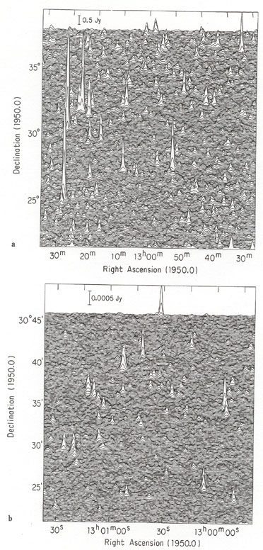 |
Figure 15.4. Profile plots of the sky near
the north galactic pole mapped with (a) the NRAO 91-m telescope (beamwidth
|
The number
n(S | )
dS of sources per steradian with flux densities
S to S + dS found in a survey made at frequency
is called the
differential source count; the total number per steradian
stronger than S,
 S
S n(s | )
ds, is called the integral source
count. Integral counts are rarely used any more because they smear rapid
changes of source density with flux density and the numbers are not
statistically independent from one flux-density level to the next
(Jauncey 1967,
Crawford et al. 1970).
The steep slopes of the differential source counts tend to obscure
features in graphical presentations, so the counts are usually either
weighted (simply multiplied
by S5/2) or normalized [divided by the count
n0(S |
) = k0
S-5/2 expected in a
static Euclidean universe; the constant k0 is usually
set so that
n(S | ) /
n0(S |
)
n(s | )
ds, is called the integral source
count. Integral counts are rarely used any more because they smear rapid
changes of source density with flux density and the numbers are not
statistically independent from one flux-density level to the next
(Jauncey 1967,
Crawford et al. 1970).
The steep slopes of the differential source counts tend to obscure
features in graphical presentations, so the counts are usually either
weighted (simply multiplied
by S5/2) or normalized [divided by the count
n0(S |
) = k0
S-5/2 expected in a
static Euclidean universe; the constant k0 is usually
set so that
n(S | ) /
n0(S |
)
 1
at S = 1 Jy] before plotting. Historically, this normalization has
been used to
facilitate comparisons with the static Euclidean count - level portions
of the actual normalized counts are said to have a "Euclidean slope,"
for example. Such comparisons can be misleading, however, because the
static Euclidean approximation
has surprisingly little relevance to the actual source counts except at
the very highest flux densities (cf.
Section 15.9). In particular, a Euclidean
slope does not signify that the sources in that flux-density range have
low redshifts or are not evolving.
1
at S = 1 Jy] before plotting. Historically, this normalization has
been used to
facilitate comparisons with the static Euclidean count - level portions
of the actual normalized counts are said to have a "Euclidean slope,"
for example. Such comparisons can be misleading, however, because the
static Euclidean approximation
has surprisingly little relevance to the actual source counts except at
the very highest flux densities (cf.
Section 15.9). In particular, a Euclidean
slope does not signify that the sources in that flux-density range have
low redshifts or are not evolving.
Source counts covering a wide range of flux densities are currently
available at
= 0.408, 0.61, 1.4, 2.7, and
5 GHz (cf.
Condon 1984b).
The most extensive is at
= 1.4 GHz and is shown in
Figure 15.5. The NRAO 91-m telescope was used to
measure the flux densities of sources stronger than S = 2 Jy at
= 1.4 GHz
(Fomalont et al. 1974)
and also in the
0.175  S < 2 Jy range
(Machalski 1978).
The fainter levels are based on VLA "snapshot" surveys
(Condon et al. 1982b,
Mitchell 1983;
Coleman et al. 1985),
the WSRT deep survey of the Lynx area
(Oort 1987),
and the deepest VLA survey
(Mitchell and Condon
1985).
The sky densities of sources too faint to be detected and counted
individually in the latter survey
were estimated statistically from their contribution to the map
fluctuation or "P(D)" distribution
(Scheuer 1957,
1974,
Condon 1974)
and are indicated by the shaded region extending down to S = 10
µJy. The integrated
emission from extragalactic sources can be used to constrain the source
count at even fainter levels. After subtracting galactic emission,
Bridle (1967)
obtained T 30
K at = 178 MHz, corresponding
to T 0.1 K at
= 1.4
GHz. The contribution
T(S) = [c2 / (2k
2)]
S
sn(s) ds from sources
stronger than S = 10 µJy is about
0.08 K, so the bulk of the extragalactic background can be accounted for
by known source populations.
S < 2 Jy range
(Machalski 1978).
The fainter levels are based on VLA "snapshot" surveys
(Condon et al. 1982b,
Mitchell 1983;
Coleman et al. 1985),
the WSRT deep survey of the Lynx area
(Oort 1987),
and the deepest VLA survey
(Mitchell and Condon
1985).
The sky densities of sources too faint to be detected and counted
individually in the latter survey
were estimated statistically from their contribution to the map
fluctuation or "P(D)" distribution
(Scheuer 1957,
1974,
Condon 1974)
and are indicated by the shaded region extending down to S = 10
µJy. The integrated
emission from extragalactic sources can be used to constrain the source
count at even fainter levels. After subtracting galactic emission,
Bridle (1967)
obtained T 30
K at = 178 MHz, corresponding
to T 0.1 K at
= 1.4
GHz. The contribution
T(S) = [c2 / (2k
2)]
S
sn(s) ds from sources
stronger than S = 10 µJy is about
0.08 K, so the bulk of the extragalactic background can be accounted for
by known source populations.
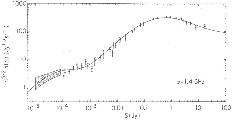 |
Figure 15.5. Weighted source count at
|
Most sources found in low-frequency surveys have power law spectra with
spectral indices near  + 0.8, but some have
the more complex spectra and lower spectral indices
(
0)
indicative of synchrotron self-absorption in compact
(
+ 0.8, but some have
the more complex spectra and lower spectral indices
(
0)
indicative of synchrotron self-absorption in compact
( < 0."01)
high-brightness (T
1011
K) components. These two source types are
effectively distinguished by the simple criterion
< 0."01)
high-brightness (T
1011
K) components. These two source types are
effectively distinguished by the simple criterion
 0.5 ("steep-spectrum" source)
or < 0.5
("flat-spectrum" source). The flat-spectrum sources
can usually be identified with quasars, while most steep-spectrum
sources are associated with
galaxies (or empty fields if the galaxies are too distant). Many
flat-spectrum sources vary in both intensity and structure on time
scales of years, and their apparent
luminosities may be affected by relativistic beaming (see Chapter
13). The evolutionary histories of these two source types may also
differ. Being so compact,
flat-spectrum sources are probably less sensitive than extended
steep-spectrum sources to changes in the average density of the
intergalactic medium or in the
energy density of the microwave background radiation with cosmological
epoch
(Rees and Setti 1968).
Finally, flat-spectrum sources can be seen at greater redshifts
because they are not so strongly attenuated by the
(1 + z)1+
Doppler term in
Equation (15.1). For these reasons, it is worthwhile to separate the
steep- and flat-spectrum sources and count them independently when
possible. The numbers of flat-spectrum
( < 0.5) and
steep-spectrum (
0.5)
sources are comparable
in high-frequency samples, and their counts at 5 GHz are plotted
separately in Figure 15.6. The data were taken from
Pauliny-Toth et
al. (1978),
Condon and Ledden (1981),
Owen et al. (1983), and
Fomalont et al. (1984).
0.5 ("steep-spectrum" source)
or < 0.5
("flat-spectrum" source). The flat-spectrum sources
can usually be identified with quasars, while most steep-spectrum
sources are associated with
galaxies (or empty fields if the galaxies are too distant). Many
flat-spectrum sources vary in both intensity and structure on time
scales of years, and their apparent
luminosities may be affected by relativistic beaming (see Chapter
13). The evolutionary histories of these two source types may also
differ. Being so compact,
flat-spectrum sources are probably less sensitive than extended
steep-spectrum sources to changes in the average density of the
intergalactic medium or in the
energy density of the microwave background radiation with cosmological
epoch
(Rees and Setti 1968).
Finally, flat-spectrum sources can be seen at greater redshifts
because they are not so strongly attenuated by the
(1 + z)1+
Doppler term in
Equation (15.1). For these reasons, it is worthwhile to separate the
steep- and flat-spectrum sources and count them independently when
possible. The numbers of flat-spectrum
( < 0.5) and
steep-spectrum (
0.5)
sources are comparable
in high-frequency samples, and their counts at 5 GHz are plotted
separately in Figure 15.6. The data were taken from
Pauliny-Toth et
al. (1978),
Condon and Ledden (1981),
Owen et al. (1983), and
Fomalont et al. (1984).
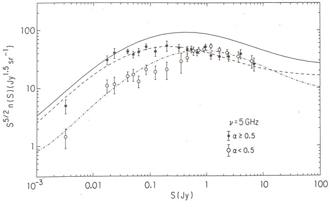 |
Figure 15.6. Weighted counts of
steep-spectrum ( |