


The parametric description of the stellar luminosity PDF is the one used by far the most often, although usually only the mean value of the distribution is computed. In fact, when we weight the stellar luminosity along an isochrone with an IMF in an SSP, it is such a mean value, µ1'(ℓi), that is obtained (see Cerviño and Luridiana 2006 for more details).
We can also evaluate by how much the possible
ℓi values differ from the mean value. For example, the
variance
µ2(ℓi), which is the average of
the square of the distance to the mean (i.e. e integral of
(ℓi -
µ1'(ℓi))2
 (ℓi) over the possible
ℓi values). In general, we can compute the difference
between the mean and the possible
ℓi elements of the distribution using any power,
(ℓi -
µ1'(ℓi))n,
and the resulting parameter is called the central n-moment,
µn(ℓi). We can also obtain the
covariance for two different luminosities
ℓi and
ℓj by computing (ℓi -
µ1'(ℓi))n(ℓj
- µ1'(ℓj))m integrated
over
(ℓi,
ℓj), where linear covariance coefficients are obtained
for the case n = m = 1.
(ℓi) over the possible
ℓi values). In general, we can compute the difference
between the mean and the possible
ℓi elements of the distribution using any power,
(ℓi -
µ1'(ℓi))n,
and the resulting parameter is called the central n-moment,
µn(ℓi). We can also obtain the
covariance for two different luminosities
ℓi and
ℓj by computing (ℓi -
µ1'(ℓi))n(ℓj
- µ1'(ℓj))m integrated
over
(ℓi,
ℓj), where linear covariance coefficients are obtained
for the case n = m = 1.
Parametric descriptions of PDFs usually use few parameters: the mean,
variance, skewness,
 1(ℓi) =
µ3 / µ23/2, and
kurtosis
2(ℓi) =
µ4 / µ22
-3. Skewness is a
measure of the asymmetry of the PDF. Kurtosis can be interpreted as a
measure of how flat or peaked a distribution is (if we focus the
comparison on the central part of the distribution) or how fat the tails
of the distribution are (if we focus on the extremes) when compared to a
Gaussian distribution. For reference, a Gaussian distribution has
1 =
2 = 0. Typical values of the four parameters
and their evolution with time for an SSP case are shown in
Fig. 3 taken from
Cerviño and
Luridiana (2006).
1(ℓi) =
µ3 / µ23/2, and
kurtosis
2(ℓi) =
µ4 / µ22
-3. Skewness is a
measure of the asymmetry of the PDF. Kurtosis can be interpreted as a
measure of how flat or peaked a distribution is (if we focus the
comparison on the central part of the distribution) or how fat the tails
of the distribution are (if we focus on the extremes) when compared to a
Gaussian distribution. For reference, a Gaussian distribution has
1 =
2 = 0. Typical values of the four parameters
and their evolution with time for an SSP case are shown in
Fig. 3 taken from
Cerviño and
Luridiana (2006).
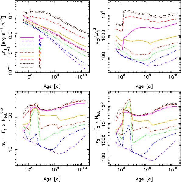 |
Figure 3. Main parameters of the luminosity
function in several photometric bands. Figure from
Cerviño and
Luridiana (2006).
In the notation used in this paper,
|
Large positive
1
values indicate that stellar
luminosity PDFs in the SSP case are L-shaped, and large positive
2
values indicate that they have fat tails. In fact,
we noted in the previous section that the stellar luminosity function is
an L-shaped distribution composed of a power-law-like component
resulting from MS stars and a fat tail at large luminosities because of
PMS stars. However,
1
and
2
computation provides us with a quantitative
characterization of the distribution shape without an explicit
visualization.
The parameters that describe the distribution of integrated
luminosities,
 (L1, ...,Ln;
tmod), are related to those of the stellar luminosity
function by simple scale relations
(Cerviño and
Luridiana 2006):
(L1, ...,Ln;
tmod), are related to those of the stellar luminosity
function by simple scale relations
(Cerviño and
Luridiana 2006):
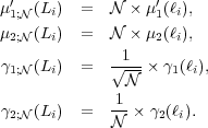 |
(1) (2) (3) (4) |
We can then obtain additional scale relations for the effective number
of stars at a given luminosity, Neff;
(Li)
(Buzzoni 1989),
the SBF,  (Tonry and Schneider
1988,
Buzzoni 1993),
and the correlation coefficients between two different luminosities,
(Tonry and Schneider
1988,
Buzzoni 1993),
and the correlation coefficients between two different luminosities,
 (Li, Lj):
 |
(5) (6) (7) |
Direct (and simple) computation of the parameters of the distribution
provides several interesting results. First, SBFs are a measure of the
scatter that is independent of
and can be applied to any
situation (from stellar clusters to galaxies) in fitting
techniques. Second, correlation coefficients are also invariant about
and can be included in any
fitting technique. Third, since the inverse of Neff;
(Li)
is the relative dispersion, when
→ ∞ the
relative dispersion goes to zero, although the absolute dispersion
(square root of the variance,  ) goes to infinity. Fourth, when
→ ∞,
1;(Li) and
2;(Li) goes to zero, and hence the shape
of the distribution of integrated luminosities becomes a Gaussian-like
distribution (actually an n-dimensional Gaussian distribution
including the corresponding
(Li, Lj)
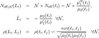
coefficients). We can also obtain the range of
1;(Li) and
2;(Li) values for which the distribution
can be approximated by a Gaussian or an expansion of Gaussian
distributions (such an Edgeworth distribution) for a certain luminosity
interval. As reference values, the shape of PDFs where
1; < 0.3 or
2; < 0.1 are well described with these four parameters by
an Edgeworth distribution; when
1; < 0.03 and
2; <
0.1, the PDFs are well described by a Gaussian distribution with the
corresponding mean and variance. A Monte Carlo simulation or a
convolution process is needed in other situations. The possible
situations are shown in Fig. 4, taken from
Cerviño and
Luridiana (2006).
) goes to infinity. Fourth, when
→ ∞,
1;(Li) and
2;(Li) goes to zero, and hence the shape
of the distribution of integrated luminosities becomes a Gaussian-like
distribution (actually an n-dimensional Gaussian distribution
including the corresponding
(Li, Lj)
coefficients). We can also obtain the range of
1;(Li) and
2;(Li) values for which the distribution
can be approximated by a Gaussian or an expansion of Gaussian
distributions (such an Edgeworth distribution) for a certain luminosity
interval. As reference values, the shape of PDFs where
1; < 0.3 or
2; < 0.1 are well described with these four parameters by
an Edgeworth distribution; when
1; < 0.03 and
2; <
0.1, the PDFs are well described by a Gaussian distribution with the
corresponding mean and variance. A Monte Carlo simulation or a
convolution process is needed in other situations. The possible
situations are shown in Fig. 4, taken from
Cerviño and
Luridiana (2006).
 |
Figure 4. Characterization of a PDF based
on Edgeworth's approximation to the second order and a Gaussianity
tolerance interval of ± 10%. Figure taken from
Cerviño and
Luridiana (2006),
where |
Another possibility that covers situations for higher
1;
and 2; values quoted here (i.e. asymmetric PDFs) is to approximate
(ℓi) by gamma distributions, as done by
Maíz
Apellániz (2009).
This approach can be used in a wide variety of situations as long as the
PDF has no bumps or the bumps are smooth enough and an accurate
description of the tails of the distribution is not required.
3.1. The mean and variance obtained using standard models
We have seen that using Eq. (1), the mean value can be expressed for any
possible value or for any
quantity related to . Most
population synthesis codes use the mass of gas transformed into stars or
the star formation rate (also expressed as the amount of mass
transformed into stars over a time interval) instead of referring to the
number of stars. Hence, the typical unit of luminosity is [erg
s-1
M -1]
or something similar. However, here I argue that the computed value
actually refers to the mean value of
ℓ(ℓ), so the units of the
luminosity obtained by the codes should be [erg s-1] and
refer to individual stars.
-1]
or something similar. However, here I argue that the computed value
actually refers to the mean value of
ℓ(ℓ), so the units of the
luminosity obtained by the codes should be [erg s-1] and
refer to individual stars.
In fact, the difference is in the interpretation and algebraic
manipulation of
 (m0,
t, Z) and the IMF. The usual argument has two distinct
steps. (1) The integrated luminosity and total stellar mass in a system
are the sum of the luminosities and masses of all the individual stars
in the system. Thus, the ratio of luminosity to mass produces the
mass-luminosity relation for the system. (2)
(m0,
t, Z) (or the IMF) provides the actual mass of the
individual stars in the system, and since the shape of such functions is
independent of the number of stars in the system, the previous
mass-luminosity relations are valid for any ensemble of stars with
similar
(m0,
t, Z) functional form. The first step is always true as
long as we know the masses and evolutionary status of all the stars in
the system (actually it is the way that each individual Monte
Carlo simulation obtains observables). The second step is false: we
do not know the individual stars in the system. We can describe the
set using a probability distribution, and hence we can describe the
integrated luminosity of all possible combinations of a sample of
individual stars.
(m0,
t, Z) and the IMF. The usual argument has two distinct
steps. (1) The integrated luminosity and total stellar mass in a system
are the sum of the luminosities and masses of all the individual stars
in the system. Thus, the ratio of luminosity to mass produces the
mass-luminosity relation for the system. (2)
(m0,
t, Z) (or the IMF) provides the actual mass of the
individual stars in the system, and since the shape of such functions is
independent of the number of stars in the system, the previous
mass-luminosity relations are valid for any ensemble of stars with
similar
(m0,
t, Z) functional form. The first step is always true as
long as we know the masses and evolutionary status of all the stars in
the system (actually it is the way that each individual Monte
Carlo simulation obtains observables). The second step is false: we
do not know the individual stars in the system. We can describe the
set using a probability distribution, and hence we can describe the
integrated luminosity of all possible combinations of a sample of
individual stars.
It is trivial to see that the mass normalisation constant used in most
synthesis codes is actually the mean stellar mass
µ'1(m0) obtained using the IMF
as a PDF.
2
Equivalently, total masses or star formation rates obtained using
inferences from synthesis models are actually
×
µ'1(m0) and
×
µ'1(m0) ×
t-1. Usually, this difference has no implication;
however, it is different to say that a galaxy has a formation rate of,
say, 0.1 stars per year (it forms, on average, a star every 10 years
whatever its mass) than 0.1
M per year
(does this mean that, on average, 103 years are needed to form a
100-M star
without forming any other star?).
Different renormalisations are performed on a physical basis, depending
on the system we are interested in. Low-mass stars in young starbursts
make almost no contribution to the UV integrated luminosity, so we can
exclude low-mass stars from the modelling. Massive stars are not present
in old systems; hence, we do not need to include massive stars in these
SSP models. The use of different normalisations can be solved easily
using a renormalisation process. Hence, we can compare the mean values
obtained from two synthesis codes that use different
constraints. However, we must be aware that
underlying any such renormalisation there are different constraints on
(m0,
t, Z), and hence there are changes in the shape of the
possible
(ℓ1, ..., ℓn;
tmod), such as the absence or presence of a Dirac
delta function at
ℓi = 0. This affects the possible values of the mean,
variance (SBF or Neft), skewness, and kurtosis used to
describe
(L1, ...,Ln;
tmod).
2 For reference, a Salpeter IMF in the
mass range 0.08-120
M has
µ'1(m0) = 0.28
M,
µ2(m0) = 1.44,
1(m0) = 1691.47, and
2(m0) = 2556.66. This
implies that the distribution of the total mass becomes Gaussian-like for
~ 3 × 10⁷
stars when the average total mass is approximately 9 ×
106
M.
Back.
 2 refers to
µ2,
2 refers to
µ2,
 1 refers to