4. STELLAR POPULATIONS USING MONTE CARLO MODELLING

Monte Carlo simulations have the advantage (and the danger) that they are easy to do and additional distributions and constraints can be included in the modelling. Fig. 5 shows the results of 10⁷ Monte Carlo simulations of SSP models with ages following a power-law distribution between 40 Myr and 2.8 Gyr, and distributed following a (discrete) power-law distribution in the range between 2 and 10⁶ stars. The figure also shows the standard modelling result using the mean value of the corresponding observable in the age range from 40 Myr to 10 Gyr.

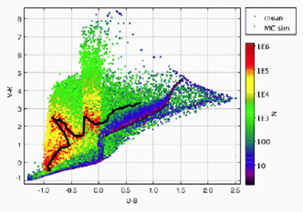Figure 5. Results of 107 Monte Carlo simulations of SSP models in the age range from 40 Myr to 2.8 Gyr, with in the range between 2 and 106 stars. The black line is the mean value of the colours obtained by a synthesis model in the age range from 40 Myr to 10 Gyr.

The first impression obtained from the plot is psychologically depressing. We had developed population synthesis codes to draw inferences from observational data, and the Monte Carlo simulations show so large a scatter that we wonder if our inferences are correct. Fig. 6, from Popescu et al. (2012), compares the age inferences for LMC clusters using Monte Carlo simulations to sample the PDF of integrated luminosities and traditional ² fitting to the mean value of the PDF (traditional synthesis model results). The figure shows a systematic discrepancy at young ages. Such an effect was also found by Fouesneau et al. (2012) for M83 stellar clusters and by Fouesneau and Lançon (2010), Silva-Villa and Larsen (2011) (among others) when trying to recover the inputs of the Monte Carlo simulations using ² fitting to the mean value obtained by parametric models. This requires stepwise interpretation. First, we must understand Monte Carlo simulation results. Second, we must figure out how to use Monte Carlo simulations to make inferences about observational data (hypothesis testing).

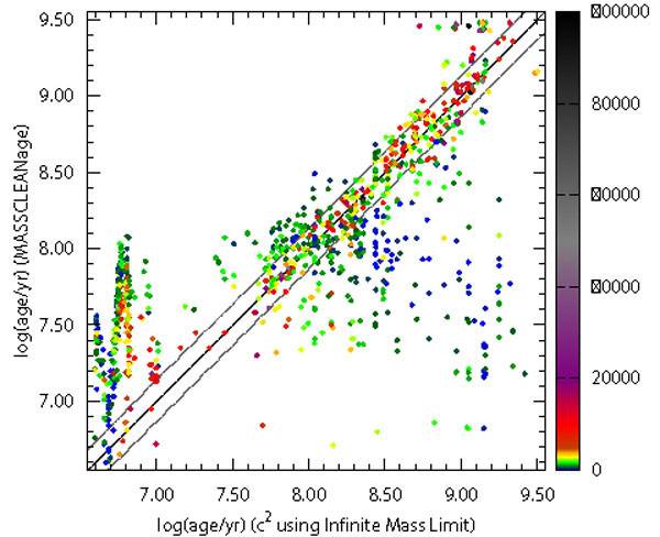Figure 6. MASSCLEAN age (Popescu and Hanson 2010b) results versus a 2 minimisation fit to the mean value obtained from SSPs for age inferences of LMC clusters. The dots are colour-coded to show the mass of the cluster. Figure from Popescu et al. (2012), who call the mean obtained by parametric models the infinite mass limit.

4.1. Understanding Monte Carlo simulations: the revenge of the stellar luminosity function

The usual first step is to analyse (qualitatively) the results for Monte Carlo simulations that implicitly represent how (L₁, ...,L_n; t_mod) varies with (Bruzual 2002, Cerviño and Valls-Gabaud 2003, Popescu and Hanson 2009, 2010a, b, Piskunov et al. 2011, Fouesneau and Lançon 2010, Silva-Villa and Larsen 2011, da Silva et al. 2012, Eldridge 2012). In general, researchers have found that at very low values, most simulations are situated in a region away from the mean obtained by parametric models; at intermediate values, the distribution of integrated luminosities or colours are (sometimes) bimodal ; at large values, the distributions become Gaussian.

The different situations are shown quantitatively in Fig. 7, taken from Cerviño (2003), which can be fully understood if we take advantage of the Monte Carlo simulations and the parametric description of synthesis models (after Gilfanov et al. 2004, Cerviño and Luridiana 2006). For ages greater than 0.1 Gyr, the figure compares when the mean bolometric luminosity of a cluster with stars, L_bol^clus = × µ₁'(ℓ_bol; t_mod), equals the maximum value of (ℓ_bol; t_mod), L_*,bol^max. This can be interpreted as the situation in which the light of a cluster is dominated by a single star, called the `lowest luminosity limit' by Cerviño and Luridiana (2004). In addition, the value needed to have, on average, at least 1 PMS star is also computed; it can be obtained using a binomial distribution over the IMF for stars below and above m_TO. The corresponding values are expressed as the mean total mass of the cluster, .

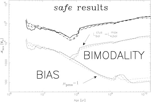Figure 7. × µ1'(m0) = ranges comparing the mean and mode of the distributions of integrated luminosities for different situations. The plots were computed for three metallicities: Z = 0.019 (solid line), Z = 0.008 (dashed line) and Z = 0.0004 (dotted dashed line). The upper line defines the value for which there are at least 10 PMS stars (t < 108 yr) or where Lbolclus > 10 × L*,bolmax (t > 108). Figure from Cerviño (2003).

From the description of (ℓt_mod) we know that the distribution is L-shaped with a modal value (maximum of the distribution) in the MS region and a mean located somewhere between the MS and PMS regions. The mean number of PMS will be less than one at low values. This means that most simulations are low-luminosity clusters composed of only MS stars, and a few simulations are high-luminosity clusters dominated by PMS stars. Here, the mode of (L; t_mod) is defined by MS stars and is biased with respect to the mean of (L; t_mod). We can also be sure that the distribution (L; t_mod) is not Gaussian-like if its mean is lower than the maximum of (ℓ ;t_mod), since the shape of the distribution is sensitive to how many luminous stars are present in each simulation (e.g. 0, 1, 2, ...) and this leads to bumps (and possibly multi-modality) in (L; t_mod). Finally, when is large, (L; t_mod) becomes Gaussian-like and the mean and mode coincide. Cerviño (2003), Cerviño and Luridiana (2004) established the maximum of (ℓ ;t_mod) 10 times to reach this safe result. Curiously, the value of that can be inferred from Fig. 7 can be used in combination with ₁ and ₂ values from Fig. 3. The resulting _1: and _2; values are approximately 0.1, the values required for Gaussian-like distributions obtained by the parametric analysis of the stellar luminosity distribution function.

This exercise shows that interpretation of Monte Carlo simulations can be established quantitatively when the parametric description is also taken into account. Surprisingly, however, except for Monte Carlo simulations used to obtain SBFs (Brocato et al. 1999, Raimondo et al. 2005, González et al. 2004), most studies do not obtain the mean or compare it with the result obtained by parametric modelling. Usually, Monte Carlo studies only verify that for large values, using relative values, the results coincide with standard models. In addition, hardly any Monte Carlo studies make explicit reference to the stellar luminosity function, nor do they compute simulations for the extreme case of = 1. Thus, psychological bias is implicit for interpretation of (m₀, t, Z) referring only to stellar clusters and synthesis models referring only to integrated properties.

Another application of the stellar luminosity function is definition of the location of simulations/observations in colour-colour diagrams (actually in any diagnostic diagram using indices that do not depend on ). Any integrated colour is a combination of the contributions of different stars; hence, individual stars define an envelope of possible colours of simulations/observations. The situation is illustrated in Fig. 8 taken from Barker et al. (2008), where the possible range of colours of individual stars and the mean of parametric synthesis models are compared.

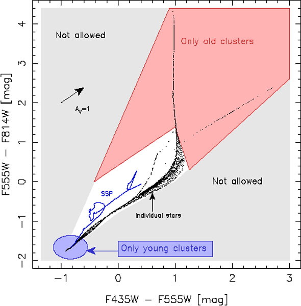Figure 8. Graphical representation of the boundary conditions. The blue track shows the mean value obtained by SSP models (from the bottom-left corner of the figure to the red colour as a function of increasing age). The red area defines the region within which only old (≥ 108 yr) clusters can reside; similarly, the blue area is the region for young (≤ 5 Myr-old) clusters. The black dots show the positions of individual stars. The grey shaded areas cannot host any clusters since there is no possible combination of single stars that can produce such cluster colours. The extinction vector for AV = 1 mag is shown for reference. Figure from Barker et al. (2008).

The final application of parametric descriptions of the integrated luminosity function to Monte Carlo simulations is a back-of-the-envelope estimation of how many Monte Carlo simulations are needed for reliable results. This number depends on the simulation objective, but a minimal requirement is that, for a fixed , the mean value obtained from the simulations (the sample mean < >) must be consistent to within an error of є of the mean obtained by the parametric modelling (the population mean). Statistics textbooks show that, independent of the shape of the distribution, the sampling mean is distributed according to a sampling distribution with variance equal to the variance of the population distribution variance divided by the sample size:

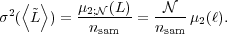(8)

Hence, expressed in relative terms, we can require that

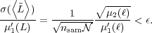(9)

We can impose a similar requirement for the variance obtained from the distribution, which results in

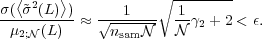(10)

An interesting result is that, for relative dispersion, the relevant parameter is the total number of stars N_tot used in the overall simulation set. Hence, the number of simulations needed to sample the distribution of integrated luminosities decreases when increases. However, for absolutes values, the ratio of to n_sam is the relevant quantity.

4.2. What we can learn from Monte Carlo simulations?

The principal advantage of Monte Carlo simulations is that they allow us to include constraints that are difficult to manage with a parametric description. Examples are constraints in the inputs (e.g. considering only simulations with a given number of stars in a given (observed) mass range, Knödlseder et al. 2002) or constraints in the outputs (e.g. considering only simulations that verify certain observational constraints in luminosities, Luridiana et al. 2003). The issue here is to compute Monte Carlo simulations and only consider those that are consistent with the desired constraints. Note that once a constraint is included, the process requires transformation of the associated probability distributions and hence a change in the parameters of the distribution, and some constraints cannot be expressed analytically as a function of input parameters. Another application that can easily be performed with Monte Carlo simulations is testing of hypotheses by comparing the distribution of the simulations and observations; examples have been described by Fumagalli et al. (2011), Eldridge (2012). Hence, this approach is ideal when fine-tuned to observational (or theoretical) constraints.

However, at the beginning of this section I stated that one of the dangers of Monte Carlo simulations is that they are easy to do. They are so easy that we can include additional distributions, such as the distribution of numbers of stars in clusters, the total mass distribution, an age distributions, without a fine-tuned specific purpose. Here, the danger is that we must understand the questions that we are addressing and how such additional distributions affect the possible inferences. For instance, Yoon et al. (2006) used Monte Carlo simulations with the typical number of stars in a globular cluster to explain bimodal distributions in globular clusters. They argued that bimodality is the result of a non-linear relation between metallicity and colour transformation. The transformation undoubtedly has an effect on the bimodality; however, the number of stars used (actually the typical number of stars that globular clusters have) is responsible for the bimodal distributions. Monte Carlo simulations using large values must converge to a Gaussian distribution.

When Monte Carlo simulations are used to obtain parameters for stellar clusters, the usual approach is to apply large grids covering the parameter space for and age. However, the situation is not as simple as expected. First, a typical situation is to use a distribution of total masses. Hence, is described by an unknown distribution. Even worse, fluctuates since the simulations must include the constraint that is an integer. Therefore, the mean values of such simulations diverge from the mean values obtained in the parametric description noted before, since they include additional distributions. Second, the inferences depend on the input distributions. For instance, Popescu et al. (2012) produced a grid assuming a flat distribution for total mass and a flat distribution in logt. They compared observational colours with the Monte Carlo grid results and obtained a distribution of the parameters (age and mass) of the Monte Carlo simulations compatible with the observations. When expressed in probabilistic terms, the grid of Monte Carlo simulations represents the probability that a cluster has a given luminosity set for given age and mass, (L | t, ), and comparison of observational data with such a set represents the probability that a cluster has a given age and mass for a given luminosity set (t, | L). The method seems to be correct, but it is a typical fallacy of conditional probabilities: it would be correct only if the resulting distribution of ages were flat in logt and if the distribution of masses were flat. The set of simulations has a prior hypothesis about the distribution of masses and ages, and the results are valid only so far as the prior is realistic. In fact, Popescu et al. (2012) obtained a distribution of ages and total masses that differs from the input distributions used in the Monte Carlo simulation set.

The situation was also illustrated by Fouesneau et al. (2012), who computed a Monte Carlo set with a flat distribution in both logt and log as priors. The authors were aware of the Bayes theorem, which connects conditional probabilities:

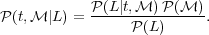(11)

They obtained age and mass distributions for observed clusters using a similar methodology to that of Popescu et al. (2012). In fact, they found that the distribution of total masses follows a power law with an exponent -2; hence, the distribution used as a prior is false. However, they claimed that the real distribution of total masses is the one obtained, similar to Popescu et al. (2012). Unfortunately, the authors were unaware that such a claim is valid only as long as a cross-validation is performed. This should involve repetition of the Monte Carlo simulations with a total mass distribution following an exponent of -2 and verification that the resulting distribution is compatible with such a prior (Tarantola 2006).

Apart from problems in using the Bayes theorem to make false hypotheses, both studies can be considered as major milestones in the inference of stellar populations using Monte Carlo modelling. Their age and total mass inferences are more realistic since they consider intrinsic stochasticity in the modelling, which is undoubtedly better than not considering stochasticity at all. The studies lack only the final step of cross-validation to obtain robust results.

Monte Carlo simulations provide two important lessons in the modelling of stellar populations that also occur in the Gaussian regime and can apply to systems of any size. The first is the problem of priors and cross-validation (i.e. an iteration of the results). The second and more important lesson is that there are no unique solutions; the best solution is actually the distribution of possible solutions. In fact, we can take advantage of the distribution of possible solutions to obtain further results (Fouesneau et al. 2012).